
The sample is the claim: representative sampling, homogeneity and what a batch result can honestly cover
Almost every figure anybody quotes about a large quantity was measured on a very small part of it. A certificate that reports a single number for four hundred grams of material was produced from perhaps twenty milligrams, which is one part in twenty thousand. The instrument that produced the number may be excellent. The analyst may be careful. None of that has any bearing on the question that decides whether the number means anything, which is whether those twenty milligrams were like the rest.
This is the least glamorous part of the work and reliably the largest source of error in it. Studies of bulk materials in industries that have measured the split, minerals, cement, grain, animal feed, have repeatedly found that the variation introduced by taking the sample is larger than the variation introduced by the analysis, often by an order of magnitude and sometimes by two. The analysis is the part that gets audited, because it leaves a paper trail. The sampling is the part that decides the answer.
What follows is a reference guide to that earlier half: naming the quantity a figure is allowed to cover, understanding why a mixture that was uniform yesterday is not uniform today, taking increments instead of a handful, choosing between random, systematic and stratified selection, deciding how many increments are enough and recognising the point where more of them add nothing, cutting a gross sample down to a test portion without changing what it represents, reading an acceptance number for what it actually promises, keeping a retention portion that is still worth something a year later, and measuring the uncertainty the sampling itself contributes rather than assuming it away.
It is written for small settings, where one or two people do everything and there is no separate sampling department. It is deliberately general. It does not describe, recommend, compare or make any claim about any material, item, treatment or substance, and it never tells a reader what to do with one.
The lot: naming what a figure is allowed to cover
Before anything is taken, one question has to be answered in writing: what exactly is this number going to be about? The answer is the lot, and everything downstream inherits its boundaries. A lot is the quantity produced or received under conditions uniform enough that a single figure can reasonably stand for all of it. That definition is doing more work than it looks: it contains a judgement about what counts as uniform, and that judgement is the first place a scheme goes wrong.
Three terms are worth keeping separate, because in ordinary speech they collapse into each other and in a report they must not.
| Term | What it is | Where it goes wrong |
|---|---|---|
| Population | The whole of the material anybody wants to know about, whether or not it is available to be sampled. | It is often larger than what was in the room. A figure gets quoted about the population when only part of it was ever present. |
| Lot | The defined quantity, bounded in time and place, that this particular figure is about. | Defined after the fact, to fit whatever was taken, or stretched to cover a second delivery that arrived later. |
| Sampling frame | The part of the lot that could actually have been reached by the person taking the sample. | Silently smaller than the lot: the back of the shelf, the bottom of the drum and the middle of the pallet were never candidates. |
The gap between the third row and the second is where most quiet failures live. A scheme can be faultless within its frame and still produce a figure that is not about the lot, because a part of the lot was never eligible to be chosen.
A usable lot definition records the boundary conditions rather than asserting uniformity. It names the start and end of the production or receipt, the identity carried on the containers, the quantity, the form the material is in, and any event during the period that could have changed conditions: a stoppage, a change of input, a change of operator, a change of temperature. If any of those happened in the middle, the honest response is usually two lots rather than one, each with its own figure.
The opposite move, merging several deliveries into one lot because they came from the same source, is convenient and expensive. It buys one certificate instead of three, and it surrenders the ability to say anything at all about any one of them. When something later turns out to be wrong with one delivery, there is no figure that applies to it, only a figure that applies to a mixture it was part of.
Homogeneity is a temporary condition
The word homogeneous is used as though it described a property of a material. It describes a relationship between a material, a scale of observation and a moment in time. A mixture can be homogeneous at the scale of a kilogram and thoroughly heterogeneous at the scale of a milligram, and the instrument only ever sees the milligram.
Two kinds of heterogeneity are worth naming separately because they behave differently and only one of them can be fixed by mixing.
- Constitutional heterogeneity is built into the material. The particles themselves differ from one another in composition or in size. No amount of stirring changes it, because stirring moves particles around without changing what any particle is. It sets a floor on how small a test portion can usefully be.
- Distributional heterogeneity is how those particles are currently arranged in space. This one does respond to mixing, and it also undoes itself again the moment mixing stops. It is the reason a scheme that worked last month can fail this month with the same material and the same people.
Segregation is the process by which a mixture that was uniform stops being uniform while nobody is doing anything to it. Four mechanisms account for most of it, and all four operate without assistance.
- Percolation. When a bed of particles is disturbed, even slightly, small particles fall through the gaps between large ones. Moving a container across a room is enough. The fine fraction ends up at the bottom and the coarse fraction at the top, which is precisely the part anyone opening the container will reach first.
- Trajectory segregation. When material is poured, particles of different size and density follow different paths through the air. The coarse fraction travels further and lands towards the outside of the heap; the fine fraction concentrates in the middle. A conical heap is therefore not one material, it is two arranged in a pattern.
- Elutriation. Air moving through or over the material carries the finest particles with it and deposits them elsewhere, usually on the surface, after the air stops. The top layer of a container that has been filled by pouring is often not representative of anything except the last few seconds of the fill.
- Agglomeration. Particles stick to one another, to moisture or to the walls of the container. A clump is a small region with its own composition, and if it is broken up by the scoop rather than by the mixing, its contents enter the sample all at once.
The practical consequence is that the interval between the last mixing and the taking of the sample belongs in the record. So does anything that happened in between: a transfer, a journey, a period standing in a warm room. A scheme that assumes uniformity and does not record when the assumption was last true is not a scheme, it is a hope with a procedure number.
One grab, and what it costs
The single most common sampling scheme in a small setting is to open the container and take a scoop from the top. It has two properties that make it hard to argue with on the day: it takes eleven seconds, and it produces a number that looks exactly like a number produced any other way. Nothing about the result announces how it was obtained.
What it actually measures is the top of the container, which is the region the four segregation mechanisms above have spent the longest working on. The coarse fraction is there because of percolation, the fines are there because of elutriation, and whatever was poured in last is there because it was poured in last. It is not a random part of the lot. It is the least representative part, selected reliably.
The alternative is the increment: a small portion taken from one location, with several of them taken from locations spread across the whole of the lot. Increments can then be handled in one of two ways, and the choice between them is a real decision rather than a formality.
- Kept separate. Each increment is analysed on its own. This is expensive and it is the only approach that can tell you how much the lot varies from place to place. It is the right choice when the question is whether the material is uniform at all, or when a single bad region would matter even if the average is acceptable.
- Combined into a composite. The increments are mixed and one analysis is run on the mixture. This is cheap and it estimates the average of the lot well. It destroys, in the act of mixing, every trace of the variation between the places the increments came from. A composite cannot tell you that one region was twice the others. It can only tell you that the average was slightly higher than expected, which reads as noise.
Both are legitimate. What is not legitimate is taking a composite and then writing conclusions that only separate increments could support. A composite result supports a statement about the mean of the lot. It supports no statement whatsoever about the worst part of the lot, and the worst part is usually what anybody actually wanted to know about.
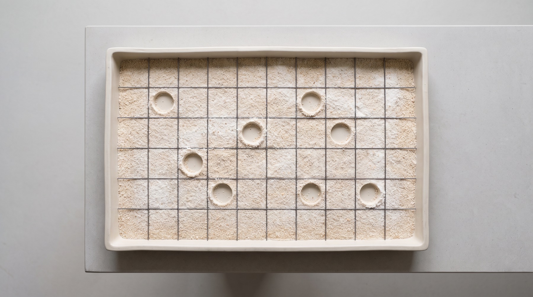
Random, systematic, stratified: choosing badly on purpose
Once it is settled that several increments will be taken, the next question is where from. There are three standard answers and each is wrong in a specific, predictable situation, which is the useful thing to know about them.
| Scheme | How positions are chosen | Fails when |
|---|---|---|
| Simple random | Every position in the lot has the same chance of being chosen, and positions are drawn independently by some mechanism that is not a person deciding. | The draw leaves whole regions untouched by chance, which is likely with a small number of increments. It is unbiased on average and can still be unlucky once. |
| Systematic | Every nth unit, or a fixed interval of time or distance, starting from one randomly chosen point. | The interval lines up with a repeating pattern in the material or the process. Then every increment lands on the same phase of the cycle and the result describes that phase, not the lot. |
| Stratified | The lot is divided into regions first, and increments are drawn within each region. | The regions are drawn around what somebody already believes, so the strata encode the assumption rather than testing it. It still guarantees coverage, which is why it is usually the right default. |
Stratified selection is the pragmatic choice for most small settings: it keeps the coverage guarantee of a systematic scheme while removing the risk that the interval synchronises with something. The strata must be written down before the material is in front of anybody.
The fourth option, the one that is used far more than the other three combined, does not appear in the table because it is not a scheme. Convenience selection is taking from wherever is reachable. It is not merely less precise. It is systematically biased in a direction that cannot be estimated afterwards, because nobody recorded which positions were reachable. Precision can be improved by taking more. Bias of this kind cannot: taking twice as much from the top gives a more precise measurement of the top.
How many increments, and where more stops buying anything
The arithmetic here is simple enough to do on paper and it settles arguments that otherwise run for years. The variance of a result has two parts that add: the variance contributed by the sampling and the variance contributed by the analysis. Written out, with s for standard deviation:
- stotal2 = ssampling2 + sanalysis2
- Taking n increments and combining them divides the sampling term by n.
- Running the analysis m times on the same material divides the analysis term by m.
Two consequences follow, and both are commonly got backwards. First, if the sampling term is the larger of the two, running the analysis in triplicate improves the total hardly at all. It improves the smaller term while leaving the larger one untouched, and it produces three numbers that agree closely with each other, which is then read as evidence that everything is fine. Close agreement between replicate analyses of the same test portion is evidence about the instrument. It is not evidence about the lot.
Second, because the sampling term falls with n rather than with n squared, the return on additional increments falls away quickly. Going from one increment to four halves the sampling standard deviation. Going from four to sixteen halves it again, and costs four times as much. Somewhere past that, the sampling term drops below the analysis term and further increments add almost nothing, because the total is by then dominated by the part that increments do not touch.
The useful version of the question is therefore not "how many is enough" in the abstract. It is: which of the two terms is currently larger, and by how much? That is measurable, and the section on uncertainty below sets out the cheapest way to measure it. Until it has been measured once, any number of increments is a guess, including the number in the procedure.
Where a scheme is stratified, the increments are usually split evenly across the strata unless there is a reason to weight them. Two reasons are legitimate: a stratum that holds more of the material deserves more increments, and a stratum known to vary more internally deserves more increments. A stratum that is simply easier to reach deserves no extra increments at all, and that is the weighting that tends to happen by itself.
From gross sample to test portion: every division is a new chance to fail
The increments are combined and there is now a gross sample, perhaps several hundred grams. The instrument needs twenty milligrams. Between those two quantities the material is reduced, usually more than once, and each reduction is itself a sampling step subject to everything above. A scheme that is careful about the first step and casual about the third has a weak link exactly where nobody is looking.
The vocabulary is worth keeping straight, because a report that uses the terms loosely cannot be checked.
| Stage | What it is | Typical scale |
|---|---|---|
| Increment | One portion taken from one position in the lot. | Grams to tens of grams |
| Gross sample | All increments taken together, before any reduction. | Hundreds of grams |
| Laboratory sample | The reduced quantity that is sent to or received by whoever will analyse it. | Tens of grams |
| Test sample | The laboratory sample after any preparation, such as grinding or drying. | Grams |
| Test portion | The quantity actually weighed out and analysed. | Milligrams |
| Retention portion | A part set aside, untouched, so the work can be revisited later. | Grams |
A certificate reports a figure measured on the test portion. Whether that figure is also about the lot depends entirely on the five rows above it.

Three methods of reduction are in common use and they are not equivalent.
- Riffle splitting. The material is poured across a series of alternating chutes that send it to two containers. Every particle meets the same series of decisions, which is why the method is insensitive to how carefully the pouring is done. It is the most reliable of the three and it halves, so reaching a quarter means two passes.
- Coning and quartering. The material is heaped into a cone, flattened, divided into four, and opposite quarters are kept. It requires no equipment. It also relies on the heap being symmetrical, and a poured heap is the textbook case of trajectory segregation, with coarse material on the outside. Done carelessly it is barely better than a scoop; done carefully it is acceptable.
- Scooping from the mixed sample. Take a spoonful from the jar after shaking it. This is the method that is almost always actually used, and it reintroduces at the last step precisely the error the increments were taken to avoid. Shaking a container of mixed particle sizes is not mixing. In many materials it is an efficient way to segregate them.
There is also a lower limit on how far reduction can go, and it comes from the material rather than from the equipment. If the test portion is small enough that it contains only a few hundred particles, then which particles happen to be in it starts to matter, and the constitutional heterogeneity described earlier turns into visible scatter between replicates. Grinding the material finer before reduction is the standard answer, because it increases the number of particles in a fixed mass. Where grinding is not possible, the honest response is to weigh out a larger test portion and to say so.
Acceptance numbers and what they actually promise
Where the question is not "what is the average" but "is this acceptable", the scheme usually becomes an attribute plan: inspect a stated number of units, count how many fail some defined criterion, and accept the lot if the count does not exceed a stated acceptance number. Two numbers therefore define the plan, the sample size and the acceptance number, and they are usually written together as something like n = 20, c = 1.
The part that is routinely misread is what c = 0 means. It does not mean the lot contains no failures. It means none were found in the units inspected. The relationship between those two statements is described by the plan's operating characteristic curve, which plots the probability of accepting the lot against the proportion of failures actually present in it. Every such curve slopes gently rather than falling off a cliff, and reading one is sobering.
A plan of n = 20, c = 0 applied to a lot in which five per cent of units would fail accepts that lot about thirty six per cent of the time. Not occasionally. Better than one time in three. To push the acceptance probability for that same lot below ten per cent, the sample size has to rise to around forty five units. Nothing about this is a defect in the plan. It is what inspecting twenty units out of a large lot can tell you, which is less than most people assume when they write c = 0 into a procedure and feel that they have been strict.
Two more terms make the curve legible, and both belong in any procedure that quotes an acceptance number:
- Producer's risk is the probability that a lot which is genuinely good enough is rejected anyway. It is the cost of the scheme to whoever supplied the material.
- Consumer's risk is the probability that a lot which is genuinely not good enough is accepted. It is the cost of the scheme to everybody downstream, and it is the number that matters when the question is whether the scheme protects anyone.
Tightened and reduced inspection exist for the same reason. A plan that switches to a larger sample after a run of rejections, and to a smaller one after a long clean run, spends effort where the evidence suggests it is needed. The switching rules have to be written down in advance, including the rule for going back, or the scheme quietly becomes "inspect less when busy".
Containers, labelling and the portion nobody opens

A sample stops being evidence the moment its identity becomes uncertain, and identity is carried by two fragile things: the label and the container.
The label is written at the moment the sample is taken, not at the end of the round. Labelling at the end of the round is the single most common cause of two samples being confidently swapped, and the swap is undetectable afterwards because both labels are legible and both are wrong. What goes on the label is the lot identity, the position or stratum the increment came from, the date and time, and who took it. What goes on the label does not include an abbreviation that only makes sense to the person writing it.
The container matters because some materials interact with some containers. Fine particles take a static charge and cling to the inside of a plastic wall, which removes a size fraction from the sample selectively. Moisture moves in or out through a closure that is not properly sealed, which changes the mass and therefore changes every figure expressed as a fraction of mass. Filling a container to the brim leaves nothing to mix in later, which forces a transfer, and a transfer is a pour, and a pour segregates.
The retention portion is the part of the scheme that costs almost nothing and is abandoned first. Its purpose is narrow and valuable: when a figure is later disputed, it allows the question to be reopened on material from the same quantity rather than on a fresh sample taken under different conditions. For it to work, it has to be taken at the same time and by the same scheme as the portion that was analysed, not scraped together afterwards from what was left. A retention portion taken from the leftovers is a sample of the leftovers.
Storage conditions and a retention period belong in the procedure, and so does a rule for disposal. An undated shelf of unlabelled jars going back four years is not an archive. It is a cupboard, and at some point somebody clears it.
Sampling uncertainty, measured rather than assumed
Most reports state an uncertainty that describes the analysis and nothing else. It is calculated from the behaviour of the instrument and the method, and it is often impressively small. It is also answering a question nobody asked, which is how much the answer would move if the same test portion were analysed again. The question that was asked is how much the answer would move if a different sample had been taken from the same lot.
That second quantity can be measured, and the cheapest way to do it is the duplicate method. It requires no new equipment and it is worth running once on any scheme that has never been checked.
- Choose eight or more lots that are typical of what is normally handled.
- On each of them, take two complete samples independently, each following the full scheme from the beginning, with positions drawn separately. Not two scoops from one gross sample: two separate runs of the whole procedure.
- Split each of those two samples and analyse both halves, so each lot yields four figures.
- The scatter between the two halves of one sample estimates the analytical variance. The scatter between the two samples, once the analytical part is subtracted, estimates the sampling variance.
The outcome is a single ratio that changes how a whole operation is run: how much of the total uncertainty comes from taking the sample, and how much from analysing it. In bulk materials that ratio commonly lands somewhere between five and one and twenty to one in favour of sampling, which means the analytical uncertainty printed on the certificate is describing the smaller half of the problem, sometimes the much smaller half.
Two things follow immediately. Effort moves to whichever term is larger, which is usually the sampling one and almost never where the budget currently goes. And any figure quoted with an uncertainty that covers only the analysis should say so in those words, because a reader is otherwise entitled to assume the interval covers the lot.
Eight failures that recur
- The lot is defined after the sample is taken. Whatever was sampled becomes, retrospectively, the thing the figure is about. It always fits, and it never tested anything.
- Increments are taken where access is easy. The scheme on paper is stratified; the scheme in practice is the top and the front. Nobody records which positions were unreachable, so the bias cannot be estimated later.
- Replicate analyses are treated as replicate samples. Three runs on one test portion agree closely, which they will, and the agreement is reported as evidence that the material is uniform. It is evidence about the instrument.
- A composite is used to answer a question about extremes. The mean is acceptable, so the lot is accepted, and a region that was twice everything else has been averaged into invisibility by design.
- The final reduction is a scoop. Everything upstream is careful. The last step before weighing is a spoon into a shaken jar, which reintroduces the whole error on the smallest quantity.
- Labels are written at the end of the round. Two samples are swapped, both labels are perfectly legible, and nothing in the record can ever reveal it.
- c = 0 is read as a guarantee. An acceptance number is treated as proof of absence rather than as a point on a curve that slopes gently and accepts bad lots at rates most readers would find surprising.
- The retention portion is what was left over. It was not taken by the scheme, so it cannot settle a dispute about the scheme, and it is usually the one part of the exercise that gets kept for years.
A ten-point check of a sampling scheme
Read a scheme against these ten questions. Each one can be answered from the written procedure and the record alone, without repeating any work. Any answer that requires somebody to remember something is a failed answer.
- Is the lot defined in writing, with its boundaries in time and quantity, before anything was taken?
- Does the record show which parts of the lot were reachable, and does the frame match the lot?
- How many increments, from how many positions, and were the positions fixed before the material was in front of anybody?
- Were the increments kept separate or composited, and does the conclusion drawn match that choice?
- When was the material last mixed or moved, and how long before sampling was that?
- By what method was the gross sample reduced, at every stage, down to the test portion?
- Is the test portion large enough to contain enough particles for the scatter between replicates to be about the method rather than about which particles were caught?
- Were labels written at the moment of taking, and do they carry lot, position, date, time and initials?
- Does the stated uncertainty cover sampling as well as analysis, and if not, does the report say so plainly?
- Was a retention portion taken by the same scheme at the same time, and can anybody still say which quantity it came from?
A scheme that answers all ten is not thereby correct. It is checkable, which is a different and more useful property. A scheme that cannot answer them produces figures whose meaning depends on who was in the room, and that dependency does not show up anywhere on the certificate.
The argument of this guide is narrow and it is not a criticism of anybody's analysis. It is that the number on a report is about the test portion, and that the chain connecting the test portion to the lot is built out of decisions that are cheap to make badly and expensive to check afterwards. Where the lot was defined, where the increments came from, how many there were, how the quantity was cut down, and what was kept back. Those decisions are made in a few minutes, by one person, usually without a record, and they set an upper limit on what any subsequent care can recover.
Which is why the sample is the claim. Everything after it can only describe what arrived.